SPD geometry utilities
robustcov.geometry provides utilities for working with symmetric positive
definite covariance and scatter matrices. These functions are useful for robust
scatter diagnostics, Tyler-style shape estimators, covariance comparison,
covariance drift monitoring, and robust input geometry.
The module is intentionally utility-focused. It does not introduce a new estimator family and does not prove convergence or optimality for every regularized scatter estimator.
Core idea
A fitted robust scatter estimator gives more than a covariance matrix. It defines a geometry on the positive-definite cone and a robust geometry on the input space.
The typical chain is:
robust scatter
     -> robust precision
     -> robust Mahalanobis distance
     -> robust similarity / kernel geometry
Information-geometry intuition
Covariance and scatter matrices are symmetric positive definite (SPD) matrices. They do not naturally live in ordinary Euclidean space. For example, taking a straight-line average of two covariance matrices is easy algebraically, but it does not always reflect the multiplicative way in which variances, correlations, condition numbers, and eigenvalue ratios change.
The SPD cone has useful geometric structure. In this geometry, two covariance matrices are compared through transformations such as
which measures how matrix B looks in the coordinate system where matrix
A has been whitened to the identity. The affine-invariant distance used in
robustcov.geometry is the Frobenius norm of the logarithm of this relative
matrix:
This distance depends on relative eigenvalue changes rather than raw coordinate differences. That makes it useful for comparing fitted covariance or scatter matrices across time windows, datasets, preprocessing choices, or regularization levels.
The log-Euclidean distance gives a simpler related view: map SPD matrices to symmetric matrices with the matrix logarithm, compare them there, and map back with the matrix exponential. This is often convenient for diagnostics and visualization.
Shape versus scale
Tyler-style scatter estimators estimate shape rather than absolute scale. If
S is a Tyler shape estimate, then multiplying S by a positive constant
describes the same shape. A normalization convention is therefore needed.
robustcov.geometry provides both common conventions:
S_trace = rcg.trace_normalize(S)
S_det = rcg.det_normalize(S)
Trace normalization fixes trace(S) = p. Determinant normalization fixes
det(S) = 1. Both are useful ways to choose a representative from the same
scale-equivalence class.
From robust scatter to robust similarity
A robust scatter estimate also defines input-space geometry. Its inverse scatter matrix gives a robust Mahalanobis distance,
This distance can be converted into a similarity function,
This is the geometric idea behind the robust kernel utilities in robustcov:
robust scatter gives robust distance, and robust distance gives robust
similarity.
What robustcov provides
robustcov.geometry is not a full information-geometry framework. It provides
a small set of practical utilities that support robust covariance workflows:
SPD matrix functions:
spd_log,spd_exp, andspd_power;SPD distances:
affine_invariant_distanceandlogeuclidean_distance;affine-invariant geodesics:
spd_geodesic;shape normalization:
trace_normalizeanddet_normalize;Tyler diagnostics:
tyler_objectiveandtyler_fixed_point_residual.
These tools make robust scatter estimates easier to compare, diagnose, and use as geometry in downstream ML tasks.
Tyler estimator as information geometry
Tyler’s shape estimator has a natural geometric interpretation. It estimates a
scatter shape rather than an absolute covariance scale. In other words,
S and c * S represent the same Tyler shape for any positive scalar
c. The natural parameter space is therefore not the full SPD cone, but the
SPD cone modulo positive rescaling.
For centered observations z_i, Tyler’s estimator depends on the directions
of the data through quadratic forms
The corresponding scale-invariant objective, up to constants, is
This objective is unchanged if S is replaced by c * S. The term
log det(S) expands or contracts volume, while the logarithmic quadratic
terms measure how the observed directions look under the inverse shape matrix.
This is the same geometry that appears in the angular central Gaussian view of Tyler’s estimator: after centering, the radial lengths of observations are discarded and the estimator fits the directional shape of the data. The result is robust to heavy tails because unusually large radii do not dominate the fit in the same way they dominate empirical covariance.
The fixed-point equation
can be read geometrically as a balance condition. Each observation contributes
a rank-one direction z_i z_i.T, but its contribution is weighted by the
inverse robust squared length under the current shape. Directions that are
already long under S receive smaller weight; directions that are short under
S receive larger weight.
Because the estimator is scale-invariant, a normalization convention is needed. For example, robustcov uses utilities such as
S_trace = rcg.trace_normalize(S)
S_det = rcg.det_normalize(S)
to choose a representative from the same scale-equivalence class.
In robustcov.geometry, this viewpoint appears directly in two diagnostic
functions:
obj = rcg.tyler_objective(S, X)
resid = rcg.tyler_fixed_point_residual(S, X)
tyler_objective evaluates the scale-invariant Tyler objective, while
tyler_fixed_point_residual measures how close a shape matrix is to the
normalized Tyler fixed-point update for a given dataset.
These functions do not make robustcov a full information-geometry package.
They expose the part of the geometry that is useful for robust covariance
workflows: shape normalization, SPD distances, geodesics, and Tyler fixed-point
diagnostics.
Basic usage
import robustcov as rc
import robustcov.geometry as rcg

est = rc.TylerShape().fit(X)

resid = rcg.tyler_fixed_point_residual(est.covariance_, X)
S_det = rcg.det_normalize(est.covariance_)
Distances on the SPD cone
d_airm = rcg.affine_invariant_distance(S1, S2)
d_log = rcg.logeuclidean_distance(S1, S2)
The affine-invariant distance is
The log-Euclidean distance is
Tyler fixed-point diagnostics
For centered observations \(z_i\), the Tyler shape fixed-point update is
tyler_fixed_point_residual reports the Frobenius distance between the
normalized update and the current shape matrix. It is a diagnostic utility, not
a formal proof of convergence for all estimator variants.
Modern ML similarity patterns
For a complete executable retrieval example, see Robust embedding retrieval / RAG filtering, which shows robust Mahalanobis reranking for a RAG-style embedding retrieval workflow.
Many modern ML systems are built around similarity scores: nearest-neighbor retrieval, reranking, attention weights, kernel methods, and embedding search. The default geometry is often Euclidean distance or cosine similarity. Those choices can work well, but they may be sensitive to anisotropic coordinates, heavy-tailed directions, sensor faults, or leverage-like embedding dimensions.
A robust scatter estimate gives an alternative geometry. If
precision = inverse(scatter), then a robust squared distance is
This distance can be used directly for ranking or converted into a similarity:
delta = x - y
d2 = delta @ precision @ delta
score = np.exp(-0.5 * d2 / length_scale**2)
The examples below are patterns, not complete models. They show where robust geometry can be inserted into existing ML workflows.
Embedding retrieval and RAG reranking
In retrieval-augmented generation or embedding search, candidates are often ranked by cosine or Euclidean similarity. If embeddings contain leverage-like directions, a few coordinates can dominate the ranking.
Robust Mahalanobis geometry can be used as a second-stage reranker:
fit = rc.FastMCD(contamination=0.05).fit(reference_embeddings)
precision = fit.precision_

def robust_distance(query, candidate):
    delta = query - candidate
    return np.sqrt(delta @ precision @ delta)

reranked = sorted(candidates, key=lambda c: robust_distance(query, c))
This does not replace semantic embedding models. Instead, it adds a robust geometry layer that can reduce the influence of atypical directions in the embedding space.
Attention over sensor windows
Attention mechanisms compare query and key vectors. In sensor or industrial monitoring, some windows may contain faults, spikes, or contaminated directions. A robust covariance estimate over normal windows can define a more stable similarity between query and key windows:
fit = rc.FastMCD(contamination=0.08).fit(normal_window_features)
precision = fit.precision_

def robust_attention_score(query, key):
    delta = query - key
    return -0.5 * delta @ precision @ delta
The resulting score can be used as a diagnostic attention-like weight or as a robust similarity feature. This is useful when raw dot products are too sensitive to faulty sensor directions.
Finance and event matching
Market states are often heavy-tailed. Event matching based on raw Euclidean distance can be distorted by shocks in a few assets or factors. Robust scatter can define a geometry for comparing market states while reducing the effect of heavy-tail leverage:
fit = rc.StudentTScatter(df=4).fit(market_state_features)
precision = fit.precision_

def state_distance(today, historical_day):
    delta = today - historical_day
    return np.sqrt(delta @ precision @ delta)
This can support tasks such as finding historical analogues, comparing volatility regimes, or constructing robust event-neighbor features.
Multimodal embeddings
Image, text, audio, and multimodal embeddings are often anisotropic: some directions carry much larger variance than others. Robust whitening or robust precision can make similarity less dominated by a small number of directions:
fit = rc.RegularizedTyler(alpha=0.10).fit(embeddings)
W = rcg.spd_power(fit.covariance_, -0.5)

embeddings_white = embeddings @ W.T
query_white = query @ W.T
After robust whitening, ordinary cosine or Euclidean similarity can be computed in the transformed space. This gives a practical bridge between robust covariance estimation and embedding-based ML workflows.
Practical notes
These patterns are most useful when the feature space is moderately sized and there are enough reference samples to estimate scatter. In higher-dimensional embedding spaces, prefer regularized estimators, dimensionality reduction, or domain-specific validation. Robust geometry should be treated as a geometry layer that improves ranking or similarity diagnostics, not as a replacement for task-level evaluation.
Geometry example gallery
Example 1: Tyler fixed-point diagnostics
This example compares two robust scatter estimates, normalizes shape matrices, computes distances on the SPD cone, and evaluates Tyler fixed-point residuals along the affine-invariant geodesic between two scatter matrices.
Run it with:
python examples/spd_geometry_diagnostics.py
Output:
SPD geometry diagnostics
------------------------
trace(S1) before normalization: 2.0
trace(trace_normalize(S1)):     2.0
det(det_normalize(S1)):         1.0

affine-invariant distance(S1, S2): 0.668446
log-Euclidean distance(S1, S2):     0.620478

Tyler fixed-point residuals
S1 on X1: 2.717e-08
S2 on X2: 8.665e-02

Geodesic from S1 to S2
t    distance_from_S1    residual_on_X1
0.00          0.000000         2.717e-08
0.25          0.167111         1.935e-02
0.50          0.334223         4.268e-02
0.75          0.501334         6.994e-02
1.00          0.668446         1.007e-01
Interpretation:
The Tyler estimate fitted on X1 has a near-zero fixed-point residual on
X1. As the geodesic moves from S1 toward the different scatter matrix
S2, the affine-invariant distance from S1 increases and the Tyler
residual on X1 increases. This illustrates how SPD geometry can be used to
compare robust scatter estimates and inspect whether a shape matrix is close to
the Tyler fixed-point equation for a given dataset.
Source excerpt:
X1 = make_heavy_tailed_data(seed=0)
X2 = make_heavy_tailed_data(seed=1)

# Add a mild regime change to X2.
X2 = X2 @ np.array([[1.2, -0.25], [0.0, 0.8]]).T

est1 = rc.TylerShape(assume_centered=True).fit(X1)
est2 = rc.RegularizedTyler(alpha=0.15, assume_centered=True).fit(X2)

S1 = est1.covariance_
S2 = est2.covariance_

print("SPD geometry diagnostics")
print("------------------------")

print("trace(S1) before normalization:", round(float(np.trace(S1)), 6))
print("trace(trace_normalize(S1)):    ", round(float(np.trace(rcg.trace_normalize(S1))), 6))
print("det(det_normalize(S1)):        ", round(float(np.linalg.det(rcg.det_normalize(S1))), 6))
print()

print("affine-invariant distance(S1, S2):", round(rcg.affine_invariant_distance(S1, S2), 6))
print("log-Euclidean distance(S1, S2):    ", round(rcg.logeuclidean_distance(S1, S2), 6))
print()

print("Tyler fixed-point residuals")
print("S1 on X1:", f"{rcg.tyler_fixed_point_residual(S1, X1):.3e}")
print("S2 on X2:", f"{rcg.tyler_fixed_point_residual(S2, X2):.3e}")
print()

print("Geodesic from S1 to S2")
print("t    distance_from_S1    residual_on_X1")
for t in np.linspace(0.0, 1.0, 5):
    S_t = rcg.spd_geodesic(S1, S2, float(t))
    d_t = rcg.affine_invariant_distance(S1, S_t)
    r_t = rcg.tyler_fixed_point_residual(S_t, X1)
    print(f"{t:0.2f} {d_t:17.6f} {r_t:17.3e}")
Example 2: ML use-case patterns
This example shows seven practical ML patterns:
covariance or regime drift monitoring across feature windows;
comparing empirical and robust scatter under contamination;
estimator stability under the same contaminated inputs;
robust similarity induced by robust scatter;
regularization-path diagnostics for Tyler-style scatter estimates;
robust whitening for preprocessing;
robust nearest-neighbor or embedding retrieval geometry.
Run it with:
python examples/spd_geometry_ml_use_cases.py
Output:
SPD geometry ML use cases
=========================

1) Robust covariance drift monitoring
window                  affine_distance_to_baseline
baseline_clean               0.1213
baseline_contaminated        0.2011
shifted_clean                2.4066
shifted_contaminated         2.4065

2) Empirical vs robust scatter under contamination
empirical covariance diag: [1.2362 2.7985]
robust covariance diag:    [1.3383 0.1814]
affine distance empirical-vs-robust: 3.0156

3) Estimator stability under the same contamination
affine distance clean->corrupted empirical covariance: 3.198
affine distance clean->corrupted robust covariance:    0.1775

4) Robust similarity from robust scatter
similarity(center, nearby point):         0.9721
similarity(center, leverage-like point):  3.409e-20

5) Regularized Tyler path geometry
alpha   dist_to_tyler   condition_number   tyler_residual
 0.02         0.1289              7.175        1.198e-02
 0.05         0.2773              6.060        2.905e-02
 0.15         0.6060              4.115        8.314e-02
 0.40         1.0735              2.272        2.159e-01

6) Robust whitening for preprocessing
distance of clean whitened covariance to identity
using empirical covariance from contaminated data: 3.0744
using robust covariance from contaminated data:    0.1261

7) Robust geometry for nearest-neighbor ranking
candidate             euclidean_distance   robust_distance
true nearby point               0.1700            0.2045
leverage-like point             2.8004            8.6385
Interpretation:
Baseline windows remain close to the reference scatter, while shifted windows have much larger affine-invariant distance. The empirical covariance is visibly inflated in the contaminated direction compared with the robust covariance. When the same clean sample is corrupted, the empirical covariance moves much farther on the SPD cone than the robust covariance. The robust similarity is high for a nearby point and essentially zero for a leverage-like point. The regularization-path table shows how SPD distances, condition numbers, and fixed-point residuals can be used to inspect Tyler-style regularized scatter estimates. The whitening example shows that preprocessing based on contaminated empirical covariance can distort the clean inlier geometry, while robust whitening stays closer to the intended identity covariance. The nearest-neighbor example shows how robust Mahalanobis geometry can distinguish ordinary nearby points from leverage-like points more clearly than raw Euclidean distance.
Visual diagnostics:
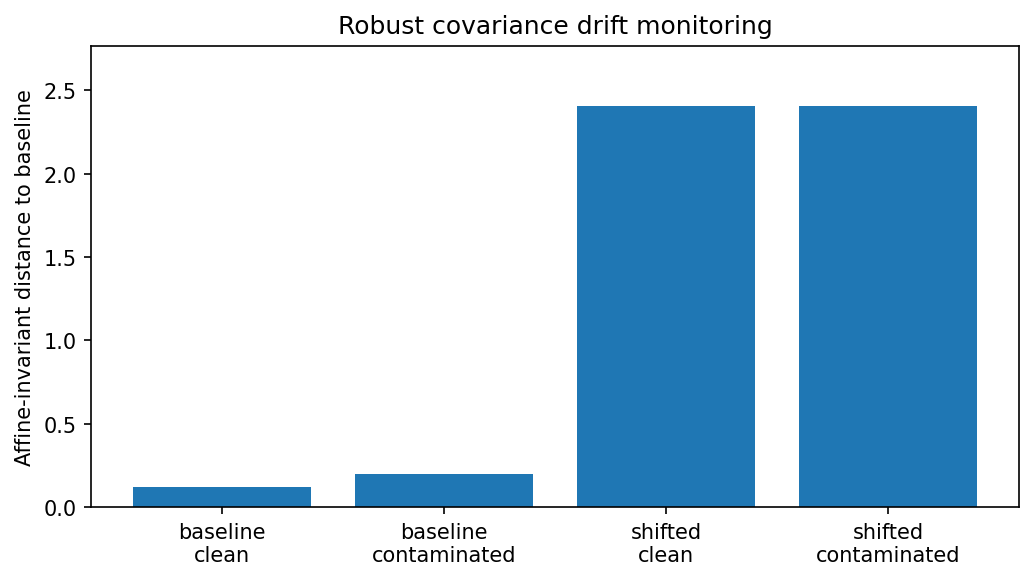
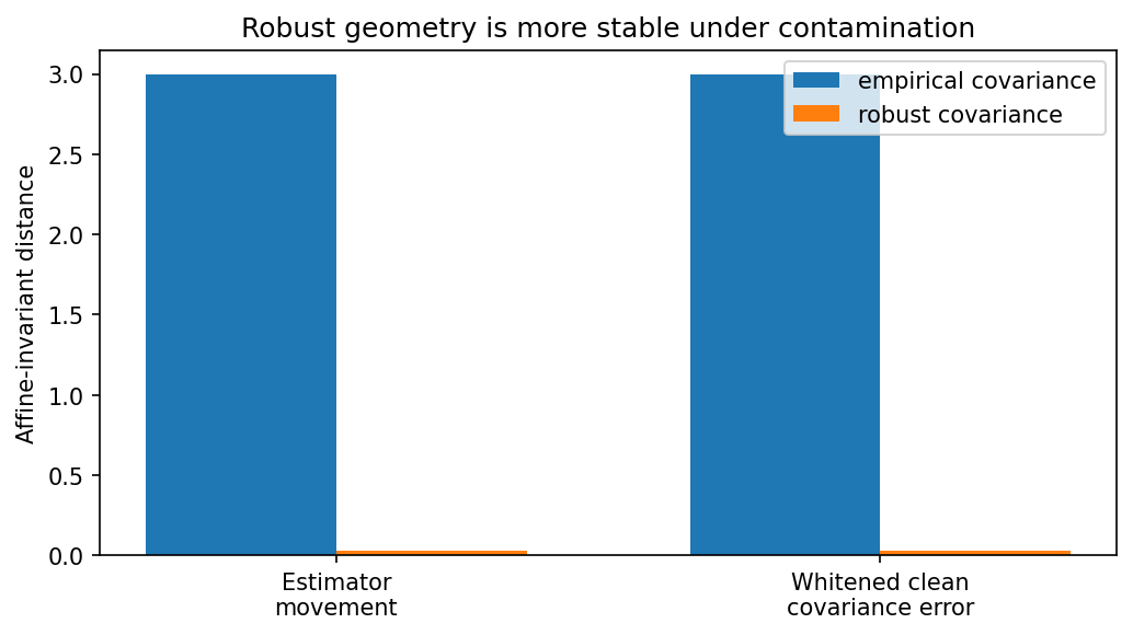
The first plot shows that covariance geometry changes little across baseline windows but changes strongly under a true shifted regime. The second plot shows that empirical covariance moves much farther under contamination and gives a worse whitening map for the clean inlier geometry.
Covariance drift monitoring
Fit a robust scatter estimate on a baseline feature window and compare later windows by affine-invariant distance:
import robustcov as rc
import robustcov.geometry as rcg

S_ref = rc.FastMCD(contamination=0.08).fit(X_baseline).covariance_
S_now = rc.FastMCD(contamination=0.08).fit(X_current).covariance_

drift_score = rcg.affine_invariant_distance(S_ref, S_now)
This gives a scalar drift score for changes in feature covariance geometry. It is useful for monitoring sensor data, embedding distributions, finance windows, or tabular ML features.
Empirical versus robust scatter
Under contamination, empirical covariance can inflate along leverage directions:
S_emp = np.cov(X, rowvar=False)
S_rob = rc.FastMCD(contamination=0.1).fit(X).covariance_

disagreement = rcg.affine_invariant_distance(S_emp, S_rob)
A large disagreement suggests that empirical covariance geometry may be strongly affected by outliers or leverage points.
Estimator stability
Geometry also gives a coordinate-aware way to compare how much an estimator moves after contamination. Fit empirical and robust scatter estimates on a clean sample and on the same sample after adding leverage points:
d_emp = rcg.affine_invariant_distance(S_emp_clean, S_emp_corrupted)
d_rob = rcg.affine_invariant_distance(S_rob_clean, S_rob_corrupted)
If d_emp is much larger than d_rob, the empirical covariance geometry is
more sensitive to the contamination.
Regularization-path diagnostics
For Tyler-style estimators, SPD distances can summarize how regularization changes the fitted scatter matrix:
S_ref = rc.TylerShape(assume_centered=True).fit(X).covariance_

for alpha in alphas:
    est = rc.RegularizedTyler(alpha=alpha, assume_centered=True).fit(X)
    d = rcg.affine_invariant_distance(S_ref, est.covariance_)
    cond = np.linalg.cond(est.covariance_)
This helps inspect the tradeoff between staying close to an unregularized shape estimate and improving numerical conditioning. The Tyler fixed-point residual is reported as a diagnostic quantity, not as a formal optimality certificate for regularized objectives.
Robust similarity
A robust scatter estimate also induces a robust similarity function. If
precision is the inverse robust covariance matrix, then
This is the same idea used by the robust GP/kernel metric utilities: robust scatter defines robust distance, and robust distance defines robust similarity.
Robust whitening for preprocessing
Covariance estimates are often used to whiten or standardize features before downstream modeling. If the covariance estimate is contaminated, the whitening map can distort the clean inlier geometry:
W_emp = rcg.spd_power(S_emp_contaminated, -0.5)
W_rob = rcg.spd_power(S_rob_contaminated, -0.5)

X_emp_white = X_clean @ W_emp.T
X_rob_white = X_clean @ W_rob.T

d_emp = rcg.affine_invariant_distance(np.eye(p), np.cov(X_emp_white, rowvar=False))
d_rob = rcg.affine_invariant_distance(np.eye(p), np.cov(X_rob_white, rowvar=False))
A smaller distance to the identity matrix means the clean inliers are closer to the intended whitened geometry.
Robust nearest-neighbor geometry
In embedding or retrieval workflows, raw Euclidean distances may not reflect the robust feature geometry. A robust precision matrix defines a Mahalanobis distance:
delta = query - candidate
robust_distance = np.sqrt(delta @ precision @ delta)
This can help distinguish ordinary nearby points from leverage-like points in directions that are atypical under the robust scatter estimate.
Source excerpt:
rng = np.random.default_rng(7)

print("SPD geometry ML use cases")
print("=========================")

# ------------------------------------------------------------------
# 1. Regime/drift detection with distances between robust scatters.
# ------------------------------------------------------------------
baseline = make_window(rng, regime="baseline", contamination=0.08)
S_ref = robust_scatter(baseline).covariance_

windows = [
    ("baseline_clean", make_window(rng, regime="baseline", contamination=0.00)),
    ("baseline_contaminated", make_window(rng, regime="baseline", contamination=0.08)),
    ("shifted_clean", make_window(rng, regime="shifted", contamination=0.00)),
    ("shifted_contaminated", make_window(rng, regime="shifted", contamination=0.08)),
]

print()
print("1) Robust covariance drift monitoring")
print("window                  affine_distance_to_baseline")
for name, X in windows:
    S = robust_scatter(X).covariance_
    d = rcg.affine_invariant_distance(S_ref, S)
    print(f"{name:24s} {d:10.4f}")

# ------------------------------------------------------------------
# 2. Empirical vs robust scatter under contaminated inputs.
# ------------------------------------------------------------------
X_contaminated = make_window(rng, regime="baseline", contamination=0.10)
S_emp = empirical_covariance(X_contaminated)
S_rob = robust_scatter(X_contaminated).covariance_

print()
print("2) Empirical vs robust scatter under contamination")
print("empirical covariance diag:", np.round(np.diag(S_emp), 4))
print("robust covariance diag:   ", np.round(np.diag(S_rob), 4))
print(
    "affine distance empirical-vs-robust:",
    round(rcg.affine_invariant_distance(S_emp, S_rob), 4),
)

# ------------------------------------------------------------------
# 3. Estimator stability under contamination.
# ------------------------------------------------------------------
X_clean = make_window(rng, regime="baseline", contamination=0.00)
X_corrupted = contaminate_same_sample(rng, X_clean, contamination=0.10)

S_emp_clean = empirical_covariance(X_clean)
S_emp_corrupted = empirical_covariance(X_corrupted)

S_rob_clean = robust_scatter(X_clean).covariance_
S_rob_corrupted = robust_scatter(X_corrupted).covariance_

d_emp = rcg.affine_invariant_distance(S_emp_clean, S_emp_corrupted)
d_rob = rcg.affine_invariant_distance(S_rob_clean, S_rob_corrupted)

print()
print("3) Estimator stability under the same contamination")
print("affine distance clean->corrupted empirical covariance:", round(d_emp, 4))
print("affine distance clean->corrupted robust covariance:   ", round(d_rob, 4))

# ------------------------------------------------------------------
# 4. Robust similarity induced by robust scatter.
# ------------------------------------------------------------------
robust_fit = robust_scatter(X_contaminated)
center = robust_fit.location_
precision = robust_fit.precision_

x_near = center + np.array([0.1, 0.1])
x_far_leverage = center + np.array([0.1, 3.5])

sim_near = robust_rbf_similarity(center, x_near, precision, length_scale=1.0)
sim_far = robust_rbf_similarity(center, x_far_leverage, precision, length_scale=1.0)

print()
print("4) Robust similarity from robust scatter")
print("similarity(center, nearby point):        ", f"{sim_near:.4f}")
print("similarity(center, leverage-like point): ", f"{sim_far:.3e}")

# ------------------------------------------------------------------
# 5. Regularization path diagnostics on the SPD cone.
# ------------------------------------------------------------------
X_path = make_window(rng, regime="baseline", contamination=0.08)
X_path = X_path - X_path.mean(axis=0)

S_tyler = rc.TylerShape(assume_centered=True).fit(X_path).covariance_

print()
print("5) Regularized Tyler path geometry")
print("alpha   dist_to_tyler   condition_number   tyler_residual")
for alpha in [0.02, 0.05, 0.15, 0.40]:
    est = rc.RegularizedTyler(alpha=alpha, assume_centered=True).fit(X_path)
    S_alpha = est.covariance_
    d_alpha = rcg.affine_invariant_distance(S_tyler, S_alpha)
    cond_alpha = np.linalg.cond(S_alpha)
    resid_alpha = rcg.tyler_fixed_point_residual(S_alpha, X_path)
    print(f"{alpha:5.2f} {d_alpha:14.4f} {cond_alpha:18.3f} {resid_alpha:16.3e}")


# ------------------------------------------------------------------
# 6. Robust whitening / preprocessing stability.
# ------------------------------------------------------------------
X_clean = make_window(rng, regime="baseline", contamination=0.00)
X_contaminated = contaminate_same_sample(rng, X_clean, contamination=0.10)

S_emp_contaminated = empirical_covariance(X_contaminated)
S_rob_contaminated = robust_scatter(X_contaminated).covariance_

W_emp = rcg.spd_power(S_emp_contaminated, -0.5)
W_rob = rcg.spd_power(S_rob_contaminated, -0.5)

X_clean_emp_white = X_clean @ W_emp.T
X_clean_rob_white = X_clean @ W_rob.T

S_clean_emp_white = empirical_covariance(X_clean_emp_white)
S_clean_rob_white = empirical_covariance(X_clean_rob_white)

I = np.eye(X_clean.shape[1])
d_emp_white = rcg.affine_invariant_distance(I, S_clean_emp_white)
d_rob_white = rcg.affine_invariant_distance(I, S_clean_rob_white)

print()
print("6) Robust whitening for preprocessing")
print("distance of clean whitened covariance to identity")
print("using empirical covariance from contaminated data:", round(d_emp_white, 4))
print("using robust covariance from contaminated data:   ", round(d_rob_white, 4))

# ------------------------------------------------------------------
# 7. Robust geometry for nearest-neighbor / embedding retrieval.
# ------------------------------------------------------------------
X_ref = make_window(rng, regime="baseline", contamination=0.08)
fit_ref = robust_scatter(X_ref)
center = fit_ref.location_
precision = fit_ref.precision_

query = center + np.array([0.0, 0.0])
true_neighbor = center + np.array([0.15, 0.08])
leverage_neighbor = center + np.array([0.05, 2.8])

euclidean_true = float(np.linalg.norm(query - true_neighbor))
euclidean_leverage = float(np.linalg.norm(query - leverage_neighbor))

robust_true = float(
    np.sqrt((query - true_neighbor) @ precision @ (query - true_neighbor))
)
robust_leverage = float(
    np.sqrt((query - leverage_neighbor) @ precision @ (query - leverage_neighbor))
)

print()
print("7) Robust geometry for nearest-neighbor ranking")
print("candidate             euclidean_distance   robust_distance")
print(f"true nearby point       {euclidean_true:14.4f} {robust_true:17.4f}")
print(f"leverage-like point     {euclidean_leverage:14.4f} {robust_leverage:17.4f}")