Wine class screening
This small real dataset tests robustcov on a tabular problem where class structure is present but not necessarily covariance-shaped.
Result at a glance
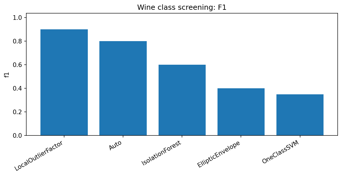
LocalOutlierFactor is best in this run with F1=0.900. robustcov Auto is second with F1=0.800 and strong ROC-AUC. This is a good example of competitive but not dominant behavior.
What the data represent
The sklearn wine dataset is reduced to a one-class screening task: one class is treated as normal and another as anomalous.
Why this estimator
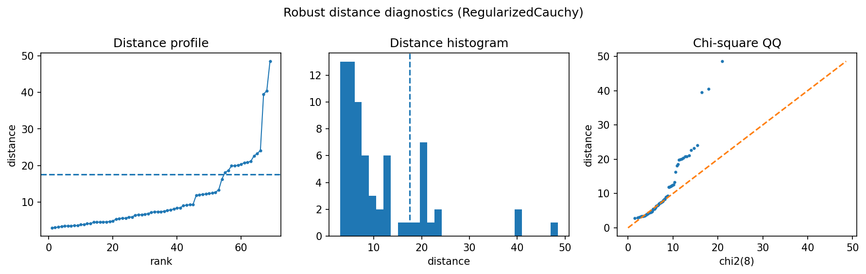
AutoRobustScatter is used because the best robust scatter choice is not obvious in advance for this small real dataset.
Reproduce the result
python examples/use_case_wine_class_screening.py
Output from the run
wine class screening
method,seconds,precision,recall,f1,roc_auc,detected
sklearn LocalOutlierFactor,0.0015,0.9000,0.9000,0.9000,0.9932,10
robustcov Auto,0.0156,0.8000,0.8000,0.8000,0.9763,10
sklearn IsolationForest,0.1131,0.6000,0.6000,0.6000,0.8949,10
sklearn EllipticEnvelope,0.0275,0.4000,0.4000,0.4000,0.9017,10
sklearn OneClassSVM,0.0010,0.3077,0.4000,0.3478,0.8627,13
normal_class=0, anomaly_class=1, anomaly_count=10, n=69, p=8, anomaly_fraction=0.145
auto_detector_estimators=3
saved diagnostics to results/use_cases/wine_class
Figures and diagnostics
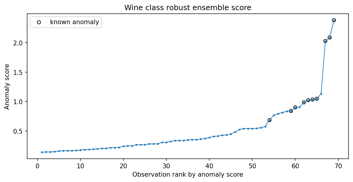
How to read the result
The baseline plot is the key figure. It shows that robustcov is useful, but that local density can be better when class separation is more neighborhood-shaped than covariance-shaped.
What this does not prove
This page is intentionally not a victory lap. It shows how to compare robustcov fairly against familiar sklearn baselines.